Conditional Formatting in Excel - Visualize Your Data

The conditional formatting in Excel offers you fascinating possibilities to make your data visually more appealing and understandable. With just a few clicks, you can ensure that important information is recognizable at a glance. In this guide, you will learn how to enhance your tables using colors, symbols, and bars. From the basics to more complex applications – let’s start with the fundamentals of conditional formatting.

Main findings

• Conditional formatting helps to highlight important data.
• You can format data based on predefined conditions with colors.
• There are various options, such as color scales, data bars, and sets of symbols, that help you visualize data in creative ways.

Step-by-step guide to conditional formatting

Start with the basics of conditional formatting to understand how to use this feature.

Step 1: Activating conditional formatting

First, open Excel and select the cells you want to format. Go to the top menu bar and click on the “Home” tab. There you will find the “Styles” group, where you will discover the option for “Conditional Formatting.” By clicking on it, a menu with various available options will open.

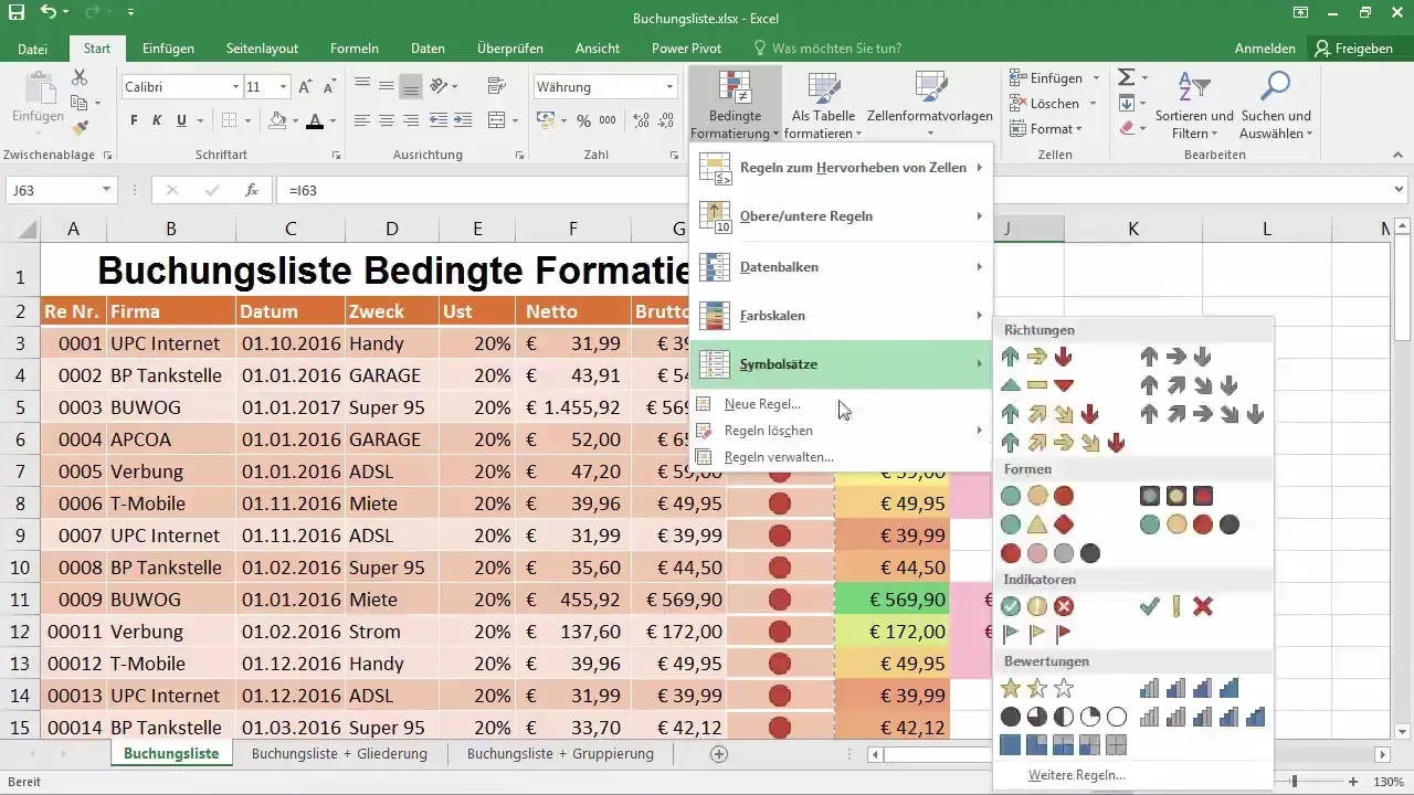
Step 2: Selecting the symbol

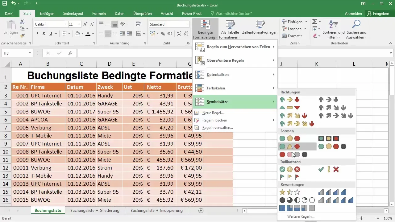
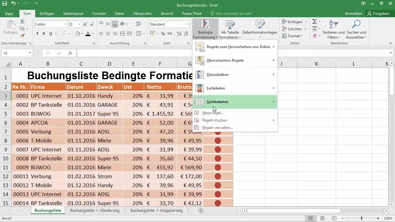
You now have the opportunity to get help through various symbols. In the menu, you can select different symbol representations. For this guide, you will use symbols in the form of circles, which will help you visually mark the values. By clicking on the circles, the formatting will be immediately applied to the selected cells.

Step 3: Rule management

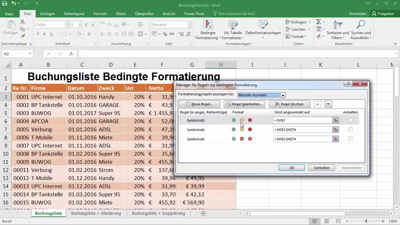
Have you selected the symbols? Then you can now adjust the formatting under “Manage Rules.” Here you will see automatically predefined rules for green, yellow, and red color values that apply to your cell selection.

Step 4: Adjusting the color values

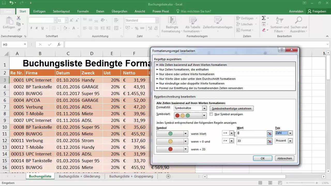
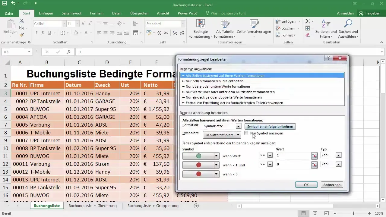
Now you can edit the rule. Click on “Edit Rule” and set the conditions under which the colors should be displayed. Set the condition that the cell will be highlighted green when the value is 1 and red when the value is less than or equal to 0.

Step 5: Adjusting the visibility of the values

To show only the symbol and not view the value, go back to rule management. Activate the option “Show only symbol.” This already adjusts the display to achieve a clear visualization.

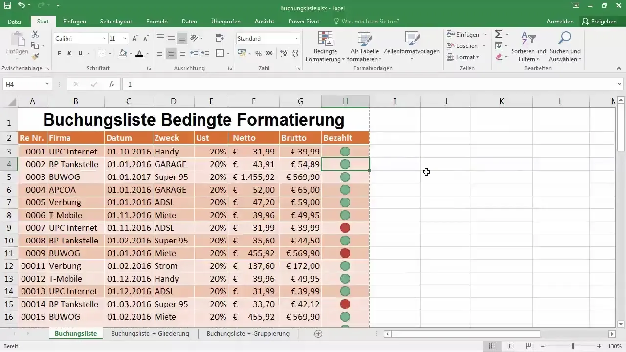
Step 6: Applying formatting to other cells

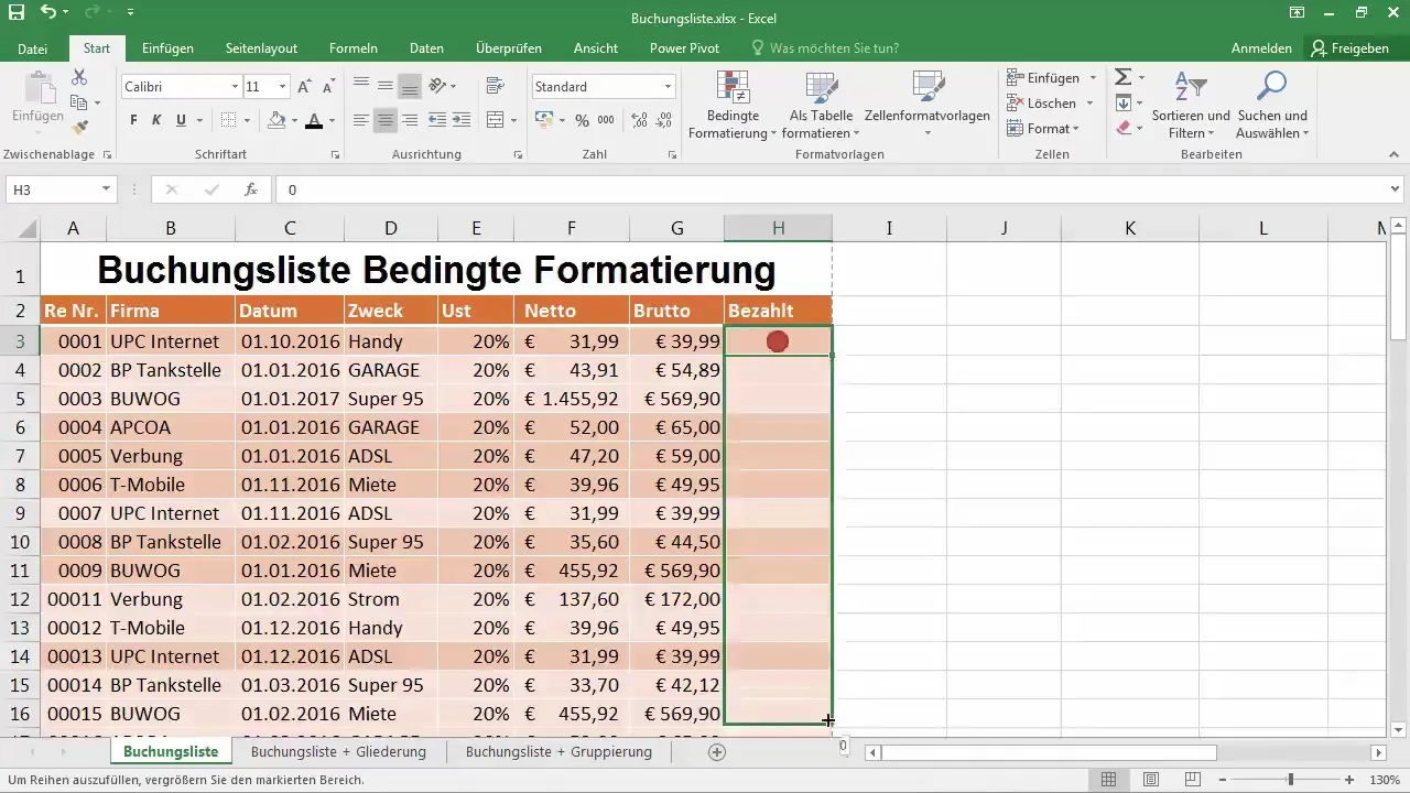
You can easily apply the newly created rule across the entire column by dragging down the formatting field. As you hover over it with your mouse, you will see how the rule is automatically applied to all cells.

Step 7: Using color scales

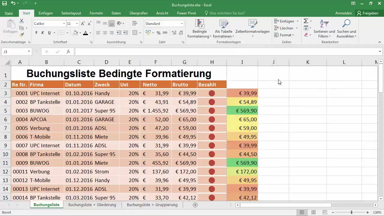
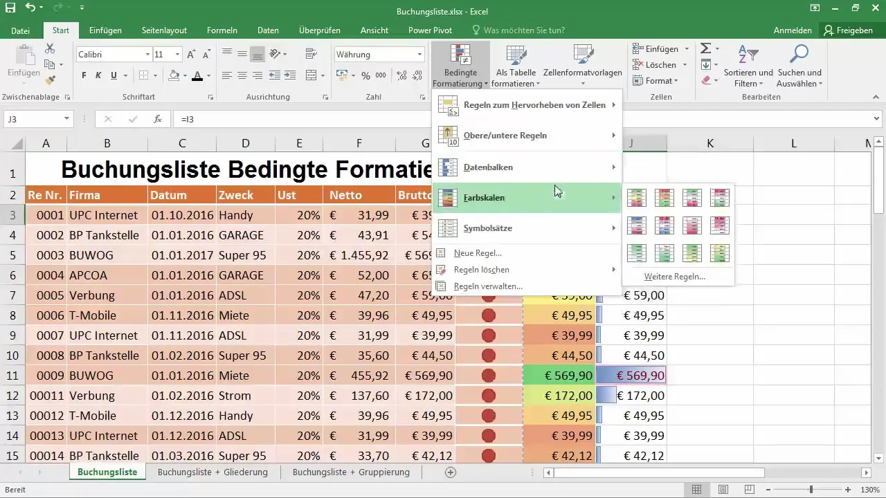
Another option for conditional formatting is color scales. Again, go to “Manage Rules.” Here you can define color scales for the data in your table. Define low, medium, and high values to visually represent the differences within your data.

Step 8: Creating data bars

To add even more dynamism to the presentation of your data, you can add data bars. These show how values compare to one another and help to quickly identify trends. Use rule management here as well to activate and display the bars.

Step 9: Optimizing the display

To ensure that your formatting does not compete with each other, open rule management and remove any that you no longer need. Check that the formatting has been correctly applied and ensure that the most important information for you is clearly highlighted.

Step 10: Experimenting with rules

Play around with different rules to optimize the design. You can set conditions that highlight the top or bottom 10% of your values or represent data comparatively. The more creative you are with the options, the more meaningful your data will be visualized.

Summary - Unleash the power of conditional formatting in Excel

Conditional formatting in Excel offers you many ways to visually highlight your data and make it more understandable. Whether you use colors, symbols, or data bars, the adjustments help you present your data optimally. With regular experimentation, you will find the best solution for you.